Getting started with jaxmat

In this tutorial, we show how to define and evaluate a simple elastoplastic behavior with nonlinear isotropic hardening.

We first import jax and may specify whether we want to run on the CPU or the GPU. We will also need the equinox package from which we use Modules to define the different behavior bricks, see more details on the use of equinox.Module..

import equinox as eqx
import jax
import jax.numpy as jnp
import matplotlib.pyplot as plt

import jaxmat.materials as jm
from jaxmat.tensors import SymmetricTensor2

jax.config.update("jax_platform_name", "cpu")

Defining a behavior

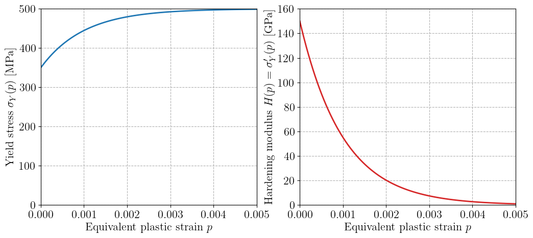
In the jaxmat.materials module, various material models such as elasticity or von Mises plasticity are already available. We will use LinearElasticIsotropic for the elastic part and vonMisesIsotropicHardening for the elastoplastic model. The latter expects a yield stress module representing the isotropic hardening. In the following, we use a Voce-type exponential hardening:

\[ \sigma_\text{Y}(p) = \sigma_0 + (\sigma_\text{u}-\sigma_0)\exp(-bp) \]

where \(\sigma_0\) (resp. \(\sigma_u\)) is the initial (resp. final) yield stress and \(b\) is a hardening parameter controlling the rate of convergence from \(\sigma_0\) to \(\sigma_u\) as a function of the cumulated plastic strain \(p\).

For this purpose, we simply define an equinox.Module with the material parameter attributes \((\sigma_0,\sigma_u, b)\) and a __call__ function which evaluates the current yield stress as a function of the cumulated plastic strain \(p\).

elasticity = jm.LinearElasticIsotropic(E=200e3, nu=0.25)


class VoceHardening(eqx.Module):
    sig0: float
    sigu: float
    b: float

    def __call__(self, p):
        return self.sig0 + (self.sigu - self.sig0) * (1 - jnp.exp(-self.b * p))


hardening = VoceHardening(sig0=350.0, sigu=500.0, b=1e3)

We now define the final material behavior of type vonMisesIsotropicHardening. We can check that it is a module containing an elasticity submodule and a yield_stress submodule. Each of these submodule holds its own material properties. The elastic submodule also allows to access the material elastic shear modulus for instance, which is 80 GPa here.

material = jm.vonMisesIsotropicHardening(elasticity=elasticity, yield_stress=hardening)
print(material)
print(material.elasticity.__dict__)
print(material.yield_stress.__dict__)

mu = elasticity.mu
print(f"\nShear modulus = {1e-3 * mu} GPa")

vonMisesIsotropicHardening(
  internal_type=jaxmat.materials.elastoplasticity.InternalState,
  elasticity=LinearElasticIsotropic(E=f64[], nu=f64[]),
  yield_stress=VoceHardening(sig0=350.0, sigu=500.0, b=1000.0)
)
{'E': Array(200000., dtype=float64), 'nu': Array(0.25, dtype=float64)}
{'sig0': 350.0, 'sigu': 500.0, 'b': 1000.0}

Shear modulus = 80.0 GPa

Since hardening is a JAX function, we can also compute its derivative using jax.grad to obtain the corresponding hardening modulus. Below, we evaluate this modulus on an array of values of cumulated plastic strain and plot the result.

hardening_modulus = jax.grad(hardening)

p = jnp.linspace(0, 5e-3, 100)
H = jax.vmap(hardening_modulus)


plt.figure(figsize=(12, 5))
plt.subplot(1, 2, 1)
plt.plot(p, hardening(p), "-C0")
plt.gca().set_ylim(bottom=0)
plt.xlabel("Equivalent plastic strain $p$")
plt.ylabel(r"Yield stress $\sigma_Y(p)$ [MPa]")
plt.subplot(1, 2, 2)
plt.plot(p, 1e-3 * H(p), "-C3")
plt.gca().set_ylim(bottom=0)
plt.xlabel("Equivalent plastic strain $p$")
plt.ylabel(r"Hardening modulus $H(p)=\sigma_Y'(p)$ [GPa]")
plt.show()

Mechanical states

In order to evaluate the response of a mechanical behavior, we need a mechanical state. Each material provides an init_state method to initialize its corresponding mechanical state with default initial values (usually 0). Below, we see that the present state contains a strain and a stress, each of them being a symmetric 2nd-rank tensor, see here for more details on tensors in jaxmat.. In addition, it also contains an internal field, which is itself a state consisting of many internal state variables. In the present case, both the cumulated plastic strain \(p\) and the total plastic strain \(\bepsp\) are declared as internal state variables.

state = material.init_state()
print(state.__dict__)
internal_state_variables = state.internal
print(internal_state_variables.__dict__)

{'internal': InternalState(
  p=f64[],
  epsp=SymmetricTensor2(
    dim=3,
    rank=2,
    base_tensor_shape=(3, 3),
    base_array_shape=(6,),
    _tensor_indices=(i64[6], i64[6]),
    _weights=f64[6],
    _array=f64[6]
  )
), 'strain': [[0. 0. 0.]
 [0. 0. 0.]
 [0. 0. 0.]], 'stress': [[0. 0. 0.]
 [0. 0. 0.]
 [0. 0. 0.]]}
{'p': Array(0., dtype=float64), 'epsp': [[0. 0. 0.]
 [0. 0. 0.]
 [0. 0. 0.]]}

from jaxmat.tensors import SymmetricTensor4  # noqa: E402

gamma = 1e-3
new_eps = jnp.array([[0, gamma / 2, 0], [gamma / 2, 0, 0], [0, 0, 0]])
new_eps = SymmetricTensor2(tensor=new_eps)
dt = 0.0
new_stress, new_state = material.constitutive_update(new_eps, state, dt)
print(new_stress)
print(new_state.__dict__)

[[ 0. 80.  0.]
 [80.  0.  0.]
 [ 0.  0.  0.]]
{'internal': InternalState(
  p=f64[],
  epsp=SymmetricTensor2(
    dim=3,
    rank=2,
    base_tensor_shape=(3, 3),
    base_array_shape=(6,),
    _tensor_indices=(i64[6], i64[6]),
    _weights=f64[6],
    _array=f64[6]
  )
), 'strain': [[0.     0.0005 0.    ]
 [0.0005 0.     0.    ]
 [0.     0.     0.    ]], 'stress': [[ 0. 80.  0.]
 [80.  0.  0.]
 [ 0.  0.  0.]]}

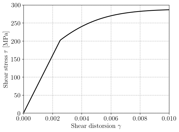
gamma_list = jnp.linspace(0, 1e-2, 100)
state = material.init_state()
tau = jnp.zeros_like(gamma_list)
for i, gamma in enumerate(gamma_list):
    new_eps = jnp.array([[0, gamma / 2, 0], [gamma / 2, 0, 0], [0, 0, 0]])
    new_eps = SymmetricTensor2(tensor=new_eps)
    dt = 0.0
    new_stress, new_state = material.constitutive_update(new_eps, state, dt)
    state = new_state
    tau = tau.at[i].set(new_stress[0, 1])

plt.plot(gamma_list, tau, "-k")
plt.xlabel(r"Shear distorsion $\gamma$")
plt.ylabel(r"Shear stress $\tau$ [MPa]")
plt.show()

tangent_operator = jax.jacfwd(material.constitutive_update, argnums=0, has_aux=True)

Let us now do the exact same calculation as before except that we call tangent_operator which now returns a tuple (Ctang, new_state) containing the tangent operator \(\mathbb{C}_\text{tang}\) and the new material state. We have formally replaced the first output of constitutive_update with its Jacobian with respect to the applied strain. As a result, the stress is not directly returned as before. We can however retrieve it from the new state as new_state.stress.

gamma_list = jnp.linspace(0, 1e-2, 100)
state = material.init_state()
tau = jnp.zeros_like(gamma_list)
p = jnp.zeros_like(gamma_list)
mu_tang = jnp.zeros_like(gamma_list)
for i, gamma in enumerate(gamma_list):
    new_eps = jnp.array([[0, gamma / 2, 0], [gamma / 2, 0, 0], [0, 0, 0]])
    new_eps = SymmetricTensor2(tensor=new_eps)
    dt = 0.0
    Ctang_arr, new_state = tangent_operator(new_eps, state, dt)
    Ctang = SymmetricTensor4(array=Ctang_arr)
    state = new_state
    new_stress = state.stress
    tau = tau.at[i].set(new_stress[0, 1])
    p = p.at[i].set(state.internal.p)
    mu_tang = mu_tang.at[i].set(Ctang[0, 1, 0, 1])

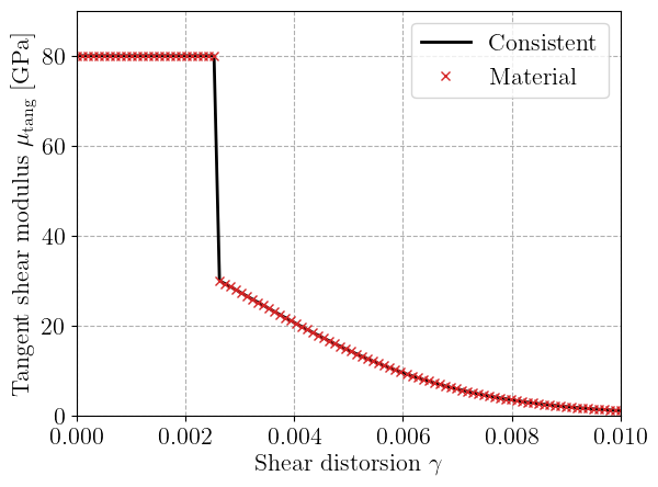
Note that the tangent operator is the derivative of a SymmetricTensor2 with respect to a SymmetricTensor2. As a result, its array representation is a \(6\times 6\) matrix. To represent it explicitly as a 4th-rank tensor, we need to wrap it as a SymmetricTensor4 object. Its component can thus be accessed as Ctang[i, j, k, l]. Collecting the value of the tangent shear modulus from Ctang[0, 1, 0, 1], its evolution clearly shows a first constant phase in the elastic regime where \(\mu_\text{tang}=\mu=80\text{ GPa}\). We see the sudden drop at the onset of plasticity which is due to the finite initial hardening slope \(R'(0)\). We know that the material (elastoplastic) tangent operator is given by:

\[\mathbb{C}^\text{ep} = 3\kappa\mathbb{J} + 2\mu\left(\mathbb{K}-\dfrac{3\mu}{3\mu+R'(p)}\boldsymbol{n}\otimes\boldsymbol{n}\right)\]

where \(\boldsymbol{n}\) is the unit normal vector in the direction of the plastic flow. For pure shear conditions, this gives the elastoplastic tangent shear modulus:

\[ \mu^\text{ep} = \mu\left(1-\dfrac{3\mu}{3\mu+R'(p)}\right) = \mu\dfrac{R'(p)}{3\mu+R'(p)} \]

plt.plot(gamma_list, mu_tang * 1e-3, "-k", label="Consistent")
mu_ep = jnp.full_like(gamma_list, mu)
plastic_points = jnp.where(p > 1e-8)
H_plast = H(p[plastic_points])
mu_ep = mu_ep.at[plastic_points].set(mu * (H_plast / (3 * mu + H_plast)))
plt.plot(gamma_list, 1e-3 * mu_ep, "xC3", label="Material")
plt.ylim(0, 90)
plt.xlabel(r"Shear distorsion $\gamma$")
plt.ylabel(r"Tangent shear modulus $\mu_\textrm{tang}$ [GPa]")
plt.legend()
plt.show()