Temperature-dependent viscoelasticity calibration

Polymer relaxation is temperature-dependent through time-temperature superposition (TTS): relaxation times shift with temperature by an Arrhenius factor, so relaxation curves at different temperatures are horizontal shifts of a single master curve. The relaxation modulus of an \(N\)-branch Prony series is

\[E(t;T) = E_\infty + \sum_i E_i\,\exp\!\Big(\!-\frac{t}{\tau_i\,a_T(T)}\Big), \qquad a_T(T) = \exp\!\Big[\frac{Q}{R}\Big(\frac1T-\frac1{T_\text{ref}}\Big)\Big].\]

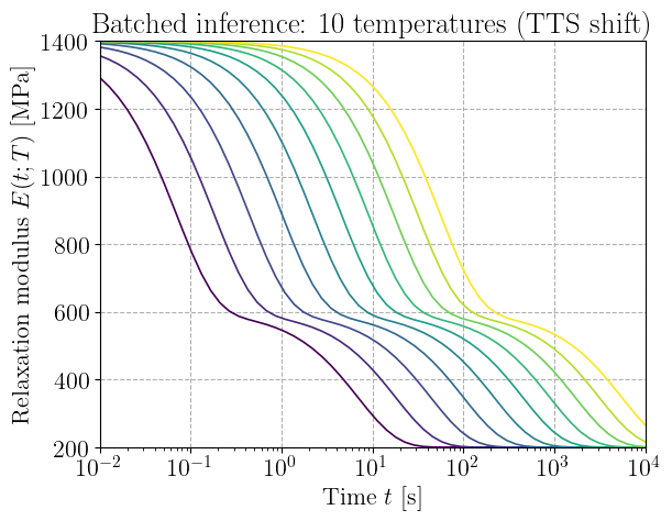
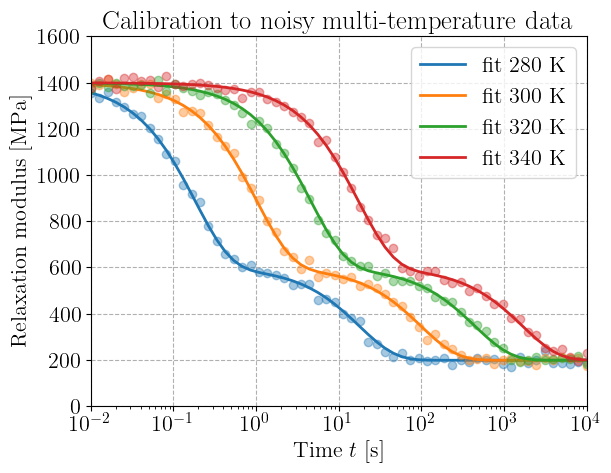
This demo shows batched inference of the response across 10 temperatures, and calibration of the temperature-dependent parameters from noisy data, using jaxmat.constraints so every physical parameter stays positive throughout.

import equinox as eqx
import jax
import jax.numpy as jnp
import matplotlib.pyplot as plt
import optax
import paramax

from jaxmat.constraints import Positive
from jaxmat.parameters import Arrhenius  # the shift-factor law

jax.config.update("jax_enable_x64", True)

Model

All moduli and times are Positive() fields (calibration cannot leave the feasible region). The Arrhenius shift factor reuses parameters.Arrhenius.

T_REF = 300.0  # K


class ThermoViscoelastic(eqx.Module):
    E_inf: jax.Array = Positive()
    E: jax.Array = Positive()  # branch moduli (vector)
    tau: jax.Array = Positive()  # reference relaxation times (vector)
    Q: jax.Array = Positive()  # activation energy for the TTS shift

    def shift(self, T):
        # a_T(T) = exp[(Q/R)(1/T - 1/T_ref)]  (Arrhenius); reuse the parameter law
        return Arrhenius(A=1.0, Q=self.Q).evaluate(T) / Arrhenius(A=1.0, Q=self.Q).evaluate(T_REF)

    def relaxation_modulus(self, t, T):
        aT = self.shift(T)
        decays = jnp.exp(-t[:, None] / (self.tau[None, :] * aT))  # (n_t, n_branch)
        return self.E_inf + decays @ self.E


def unwrap_eval(model, t, T):
    return paramax.unwrap(model).relaxation_modulus(t, T)

Ground-truth model and synthetic data

Two Prony branches with well-separated relaxation times; data are relaxation moduli measured over log-spaced time at several temperatures, plus noise.

truth = ThermoViscoelastic(
    E_inf=200.0, E=jnp.array([800.0, 400.0]), tau=jnp.array([1.0, 100.0]), Q=6.0e4
)

t = jnp.logspace(-2, 4, 60)  # time [s]
T_data = jnp.array([280.0, 300.0, 320.0, 340.0])  # measurement temperatures [K]

key = jax.random.PRNGKey(0)
clean = jax.vmap(lambda T: unwrap_eval(truth, t, T))(T_data)  # (n_T, n_t)
noise = 15.0 * jax.random.normal(key, clean.shape)
data = clean + noise

Batched inference across 10 temperatures

vmap evaluates the full relaxation curve at 10 temperatures at once – the curves shift left as temperature rises (faster relaxation), the TTS signature.

T_sweep = jnp.linspace(270.0, 360.0, 10)
curves = jax.jit(jax.vmap(lambda T: unwrap_eval(truth, t, T)))(T_sweep)
print("batched inference:", curves.shape, "(10 temperatures x", t.shape[0], "times)")

plt.figure()
for c, T in zip(curves, T_sweep):
    plt.semilogx(t, c, color=plt.cm.viridis((T - 270) / 90), lw=1.2)
plt.xlabel("Time $t$ [s]")
plt.ylabel("Relaxation modulus $E(t;T)$ [MPa]")
plt.title("Batched inference: 10 temperatures (TTS shift)")

batched inference: (10, 60) (10 temperatures x 60 times)

Text(0.5, 1.0, 'Batched inference: 10 temperatures (TTS shift)')

Calibration of the temperature-dependent parameters

In this section, we explore the calibration of the temperature-dependent viscoelastic model from the noisy data which we just generated. Starting from a wrong guess, we fit \(E_\infty, E_i, \tau_i, Q\) to the noisy multi-temperature data. Note that elastic parameters and parameters from the temperature model (here the activation energy \(Q\)) are all packed together in the global model PyTree and calibrated simultaneously.

Because every parameter is declared Positive(), the model does not store the physical values directly: it stores an unbounded latent parameter \(z_{\theta_i}\) such that \(\theta_i = \exp(z_{\theta_i}) > 0\). These latents are the differentiable leaves of the PyTree, so the optimizer operates on them and no gradient step can ever make a parameter negative. Inside the loss, paramax.unwrap is applied once to reconstruct the physical model parameters so that stresses are computed with correctly-scaled, physical parameters. Automatic differentiation then propagates the gradient back to the latent representations using the Positive \(\exp\) mapping. A useful side effect is that working in \(\log\)-space equalizes parameters spanning different orders of magnitude (here \(Q\sim10^4\), \(E\sim 100\) and \(\tau\sim 10\)), since a step in \(z_{\theta_i}\) is a relative step in \(\theta_i\). `adam(3e-2)`` is thus a ~3% relative step on each parameter, which is sensible for all of them simultaneously.

model = ThermoViscoelastic(
    E_inf=100.0, E=jnp.array([500.0, 500.0]), tau=jnp.array([3.0, 30.0]), Q=3.0e4
)


def loss(model, T_data, data):
    pred = jax.vmap(lambda T: unwrap_eval(model, t, T))(T_data)
    return jnp.mean((pred - data) ** 2)


opt = optax.adam(3e-2)
opt_state = opt.init(eqx.filter(model, eqx.is_inexact_array))


@eqx.filter_jit
def step(model, opt_state):
    loss_value, g = eqx.filter_value_and_grad(loss)(model, T_data, data)
    updates, opt_state = opt.update(g, opt_state, model)
    return eqx.apply_updates(model, updates), opt_state, loss_value


for i in range(500):
    model, opt_state, loss_value = step(model, opt_state)
    if i % 50 == 0 or i == 499:
        print(f"step {i:5d}  loss = {float(loss_value):10.2f}")

fit = paramax.unwrap(model)
tru = paramax.unwrap(truth)
print("\nparameter recovery (fitted vs true):")
print(f"  E_inf : {float(fit.E_inf):7.1f}  vs {float(tru.E_inf):7.1f}")
print(f"  E     : {[round(float(x), 1) for x in fit.E]}  vs {[round(float(x), 1) for x in tru.E]}")
print(
    f"  tau   : {[round(float(x), 2) for x in fit.tau]}  vs {[round(float(x), 2) for x in tru.tau]}"
)
print(f"  Q     : {float(fit.Q):.3e}  vs {float(tru.Q):.3e}")

step     0  loss =   44421.00
step    50  loss =     765.32
step   100  loss =     252.54
step   150  loss =     232.53
step   200  loss =     231.45
step   250  loss =     231.43
step   300  loss =     231.43
step   350  loss =     231.43
step   400  loss =     231.43
step   450  loss =     231.43
step   499  loss =     231.43

parameter recovery (fitted vs true):
  E_inf :   197.6  vs   200.0
  E     : [799.0, 401.9]  vs [800.0, 400.0]
  tau   : [1.01, 98.78]  vs [1.0, 100.0]
  Q     : 5.998e+04  vs 6.000e+04

The calibration processes converges quickly recovering the ground truth value with a very good accuracy.

Results

We now compare the prediction of the fitted model against the noisy data for comparison, showing a very good calibration accuracy.

plt.figure()
for d, T in zip(data, T_data):
    h = plt.semilogx(t, d, "o", ms=6, alpha=0.4)
    plt.semilogx(
        t, unwrap_eval(fit, t, T), "-", color=h[0].get_color(), lw=2.0, label=f"fit {int(T)} K"
    )
plt.xlabel("Time $t$ [s]")
plt.ylabel("Relaxation modulus [MPa]")
plt.title("Calibration to noisy multi-temperature data")
plt.legend()

<matplotlib.legend.Legend at 0x741b587b6ba0>

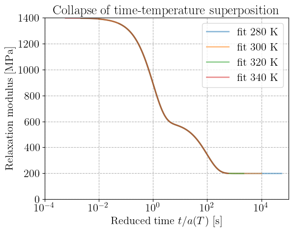
Finally, we check that the time-temperature superposition is well retried by plotting the master curve of the relaxation modulus as a function of the reduced time \(\tilde{t} = t/a(T)\).

plt.figure()
for d, T in zip(data, T_data):
    # h = plt.semilogx(t, d, "o", ms=6, alpha=0.4)
    plt.semilogx(
        t / fit.shift(T),
        unwrap_eval(fit, t, T),
        "-",
        lw=2.0,
        alpha=0.5,
        label=f"fit {int(T)} K",
    )
plt.xlabel("Reduced time $t/a(T)$ [s]")
plt.ylabel("Relaxation modulus [MPa]")
plt.title("Collapse of time-temperature superposition")
plt.legend()

<matplotlib.legend.Legend at 0x741be053d010>